XAI

Xai is a model interpretation module, which can explain how complex model prediction results are formed, and help users quickly understand the relationship between input and output. At present, the xai module is divided into two sub-modules: ante_hoc and post_hoc. The former provides interpretability based on the designed model network structure, while the latter has nothing to do with the model network, but interprets the original model through the proxy model.

1. Prepare Data

1.1. Get Data and import library

Get PaddleTS inner-build datasets.

import numpy as np
import pandas as pd
import paddle
import matplotlib.pyplot as plt

np.random.seed(123456)
paddle.seed(123456)

from paddlets import TSDataset, TimeSeries
from paddlets.xai.post_hoc.shap_explainer import ShapExplainer
from paddlets.datasets.repository import get_dataset

tsdataset = get_dataset("ECL")

1.2. Split Data

Split dataset into train/test/valid.

ts_known = TimeSeries(data[['MT_001', ]], freq='1H').copy()
ts_cols = data.columns
keep_cols = ['MT_000', ]
remove_cols = []
for col, types in ts_cols.items():
    if (types is 'target'):
        continue
    if (col not in keep_cols):
        remove_cols.append(col)

data.drop(remove_cols)
data.set_known_cov(ts_known)

data, _ = data.split('2014-06-30')
train_data, test_data = data.split('2014-06-15')
train_data, val_data = train_data.split('2014-06-01')

2. Prepare model parameters

Prepare base model parameters.

in_chunk_len = 24
out_chunk_len = 24
skip_chunk_len = 0
sampling_stride = 24
max_epochs = 10
patience = 5

3. Construct and Fitting

Construct and Fitting pipeline

from paddlets.models.forecasting import NBEATSModel
from paddlets.transform import StandardScaler
from paddlets.pipeline.pipeline import Pipeline

pipeline_list = [(StandardScaler, {}),
                 (NBEATSModel, {'in_chunk_len': in_chunk_len,
                                'out_chunk_len': out_chunk_len,
                                'skip_chunk_len': skip_chunk_len,
                                'max_epochs': max_epochs,
                                'patience': patience})
                ]
pipe = Pipeline(pipeline_list)
pipe.fit(train_data, val_data)

4. Xai

Interpretation of prediction results based on kernel shap method.

4.1. Initialize the interpreter

ShapExplainer: Help users realize the link bridge between the PaddleTS model and the shap interpreter, and better help users understand the nature of the output results.

se = ShapExplainer(pipe, train_data, background_sample_number=100, keep_index=True, use_paddleloader=False)

4.2. Explain test sample

ShapExplainer.explain: Help users calculate samples that need to be interpreted, and give feature contribution

shap_value = se.explain(test_data_fea, nsamples=100)

4.3. Feature contribution figure

ShapExplainer.force_plot: Use additive layers to show sample data time points that require interpretation. In the display results, lag_0 represents the last moment of in_chunk_len, and lag_1 represents the first moment of out_chunk_len

se.force_plot(out_chunk_indice=[5, ], sample_index=0, contribution_threshold=0.05)

fig_1

4.4. Feature importance display

ShapExplainer.summary_plot: Calculate and sort the feature contribution value for the specified time point to be predicted.

se.summary_plot(out_chunk_indice=[5, ], sample_index=0)

fig_2

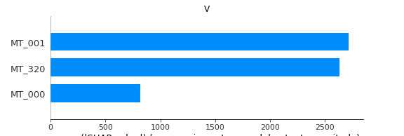
4.5. Multi-dimensional output contribution value display—feature variable

Note: The following shows the feature contribution of each feature variable at all input time steps and all output time steps

se.plot(method='V')

fig_3

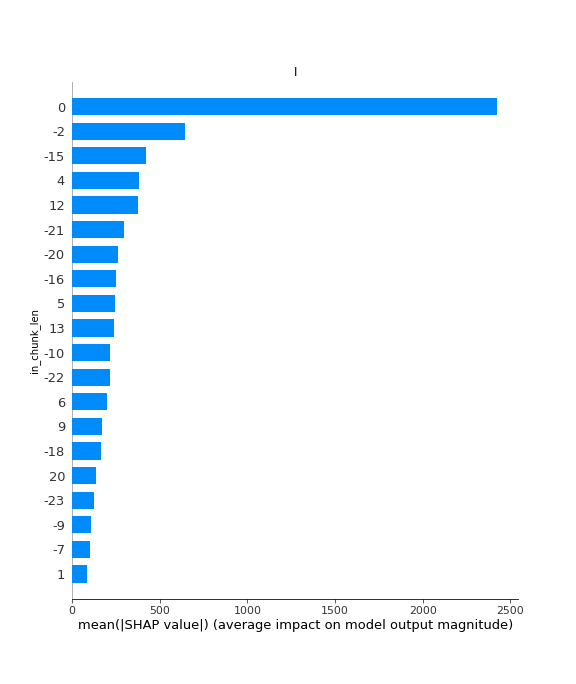
4.6. Multi-dimensional output contribution value display—input time step

Note: The following shows the feature contribution of each input time step on all features and all output time steps.

se.plot(method='I')

fig_4

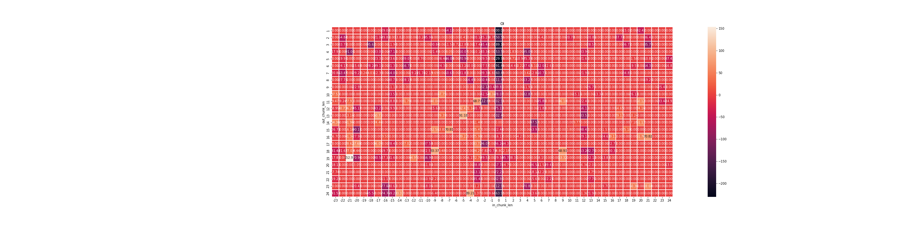
4.7. Multi-dimensional output contribution value display—Input time step and output time step

Note: The following shows the feature contribution of each input time step and each output time step on all feature variables

se.plot(method='OI')

fig_5

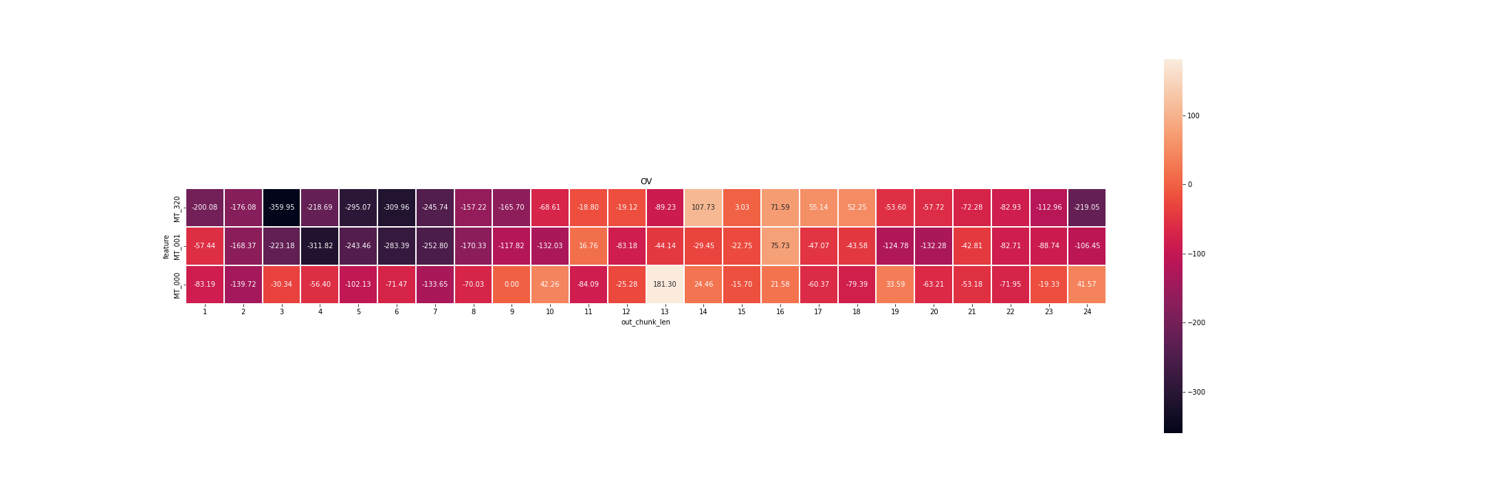
4.8. Multi-dimensional output contribution value display—Feature variables and output time steps

Note: The following shows the feature contribution of each feature variable and each output time step on all input time steps

se.plot(method='OV')

fig_6

4.9. Multi-dimensional output contribution value display—Feature variables and input time steps

Note: The following shows the feature contribution of each input time step and each variable over all output time steps

se.plot(method='IV', figsize=(30, 5))

fig_7